A Unified Theory of Randomness
Standard geometric objects can be described by simple rules — every straight line, for example, is just y = ax + b — and they stand in neat relation to each other: Connect two points to make a line, connect four line segments to make a square, connect six squares to make a cube.
These are not the kinds of objects that concern Scott Sheffield. Sheffield, a professor of mathematics at the Massachusetts Institute of Technology, studies shapes that are constructed by random processes. No two of them are ever exactly alike. Consider the most familiar random shape, the random walk, which shows up everywhere from the movement of financial asset prices to the path of particles in quantum physics. These walks are described as random because no knowledge of the path up to a given point can allow you to predict where it will go next.
Beyond the one-dimensional random walk, there are many other kinds of random shapes. There are varieties of random paths, random two-dimensional surfaces, random growth models that approximate, for example, the way a lichen spreads on a rock. All of these shapes emerge naturally in the physical world, yet until recently they’ve existed beyond the boundaries of rigorous mathematical thought. Given a large collection of random paths or random two-dimensional shapes, mathematicians would have been at a loss to say much about what these random objects shared in common.
Yet in work over the past few years, Sheffield and his frequent collaborator, Jason Miller, a professor at the University of Cambridge, have shown that these random shapes can be categorized into various classes, that these classes have distinct properties of their own, and that some kinds of random objects have surprisingly clear connections with other kinds of random objects. Their work forms the beginning of a unified theory of geometric randomness.
“You take the most natural objects — trees, paths, surfaces — and you show they’re all related to each other,” Sheffield said. “And once you have these relationships, you can prove all sorts of new theorems you couldn’t prove before.”
In the coming months, Sheffield and Miller will publish the final part of a three-paper series that for the first time provides a comprehensive view of random two-dimensional surfaces — an achievement not unlike the Euclidean mapping of the plane.
“Scott and Jason have been able to implement natural ideas and not be rolled over by technical details,” said Wendelin Werner, a professor at ETH Zurich and winner of the Fields Medal in 2006 for his work in probability theory and statistical physics. “They have been basically able to push for results that looked out of reach using other approaches.”
A Random Walk on a Quantum String
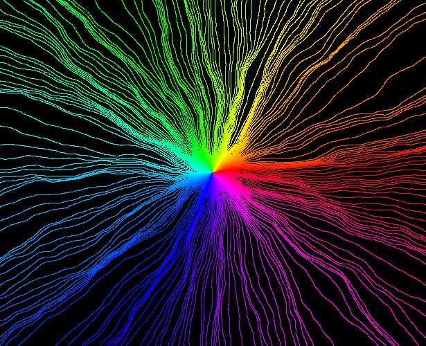
In standard Euclidean geometry, objects of interest include lines, rays, and smooth curves like circles and parabolas. The coordinate values of the points in these shapes follow clear, ordered patterns that can be described by functions. If you know the value of two points on a line, for instance, you know the values of all other points on the line. The same is true for the values of the points on each of the rays in this first image, which begin at a point and radiate outward.
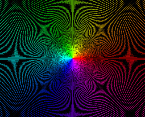
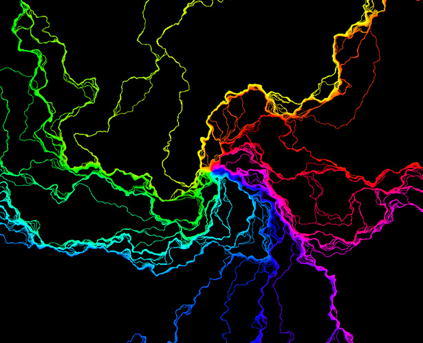
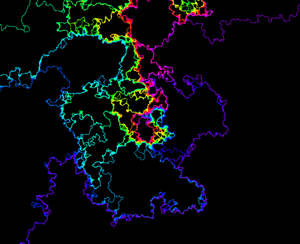
If Earth were not round, but were instead a more complicated shape, possibly curved in wild and random ways, then an airplane’s trajectory (as shown on a flat two-dimensional map) would appear even more irregular, like the rays in the following images.
The first kind of random shape to be understood in this way was the random walk. Conceptually, a one-dimensional random walk is the kind of path you’d get if you repeatedly flipped a coin and walked one way for heads and the other way for tails. In the real world, this type of movement first came to attention in 1827 when the English botanist Robert Brown observed the random movements of pollen grains suspended in water. The seemingly random motion was caused by individual water molecules bumping into each pollen grain. Later, in the 1920s, Norbert Wiener of MIT gave a precise mathematical description of this process, which is called Brownian motion.
Brownian motion is the “scaling limit” of random walks — if you consider a random walk where each step size is very small, and the amount of time between steps is also very small, these random paths look more and more like Brownian motion. It’s the shape that almost all random walks converge to over time.
Two-dimensional random spaces, in contrast, first preoccupied physicists as they tried to understand the structure of the universe.
In string theory, one considers tiny strings that wiggle and evolve in time. Just as the time trajectory of a point can be plotted as a one-dimensional curve, the time trajectory of a string can be understood as a two-dimensional curve. This curve, called a worldsheet, encodes the history of the one-dimensional string as it wriggles through time.
“To make sense of quantum physics for strings,” said Sheffield, “you want to have something like Brownian motion for surfaces.”
For years, physicists have had something like that, at least in part. In the 1980s, physicist Alexander Polyakov, who’s now at Princeton University, came up with a way of describing these surfaces that came to be called Liouville quantum gravity (LQG). It provided an incomplete but still useful view of random two-dimensional surfaces. In particular, it gave physicists a way of defining a surface’s angles so that they could calculate the surface area.
In parallel, another model, called the Brownian map, provided a different way to study random two-dimensional surfaces. Where LQG facilitates calculations about area, the Brownian map has a structure that allows researchers to calculate distances between points. Together, the Brownian map and LQG gave physicists and mathematicians two complementary perspectives on what they hoped were fundamentally the same object. But they couldn’t prove that LQG and the Brownian map were in fact compatible with each other.
“It was this weird situation where there were two models for what you’d call the most canonical random surface, two competing random surface models, that came with different information associated with them,” said Sheffield.
Beginning in 2013, Sheffield and Miller set out to prove that these two models described fundamentally the same thing.
The Problem With Random Growth
Sheffield and Miller began collaborating thanks to a kind of dare. As a graduate student at Stanford in the early 2000s, Sheffield worked under Amir Dembo, a probability theorist. In his dissertation, Sheffield formulated a problem having to do with finding order in a complicated set of surfaces. He posed the question as a thought exercise as much as anything else.
David Kaplan, Petr Stepanek and Ryan Griffin for Quanta Magazine; music by Kevin MacLeod
Nature’s Symmetries: In this 2-minute video, David Kaplan explains how the search for hidden symmetries leads to discoveries like the Higgs boson.
“I thought this would be a problem that would be very hard and take 200 pages to solve and probably nobody would ever do it,” Sheffield said.
But along came Miller. In 2006, a few years after Sheffield had graduated, Miller enrolled at Stanford and also started studying under Dembo, who assigned him to work on Sheffield’s problem as way of getting to know random processes. “Jason managed to solve this, I was impressed, we started working on some things together, and eventually we had a chance to hire him at MIT as a postdoc,” Sheffield said.
In order to show that LQG and the Brownian map were equivalent models of a random two-dimensional surface, Sheffield and Miller adopted an approach that was simple enough conceptually. They decided to see if they could invent a way to measure distance on LQG surfaces and then show that this new distance measurement was the same as the distance measurement that came packaged with the Brownian map.
To do this, Sheffield and Miller thought about devising a mathematical ruler that could be used to measure distance on LQG surfaces. Yet they immediately realized that ordinary rulers would not fit nicely into these random surfaces — the space is so wild that one cannot move a straight object around without the object getting torn apart.
The duo forgot about rulers. Instead, they tried to reinterpret the distance question as a question about growth. To see how this works, imagine a bacterial colony growing on some surface. At first it occupies a single point, but as time goes on it expands in all directions. If you wanted to measure the distance between two points, one (seemingly roundabout) way of doing that would be to start a bacterial colony at one point and measure how much time it took the colony to encompass the other point. Sheffield said that the trick is to somehow “describe this process of gradually growing a ball.”
It’s easy to describe how a ball grows in the ordinary plane, where all points are known and fixed and growth is deterministic. Random growth is far harder to describe and has long vexed mathematicians. Yet as Sheffield and Miller were soon to learn, “[random growth] becomes easier to understand on a random surface than on a smooth surface,” said Sheffield. The randomness in the growth model speaks, in a sense, the same language as the randomness on the surface on which the growth model proceeds. “You add a crazy growth model on a crazy surface, but somehow in some ways it actually makes your life better,” he said.
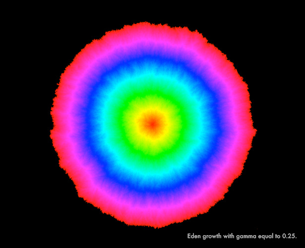
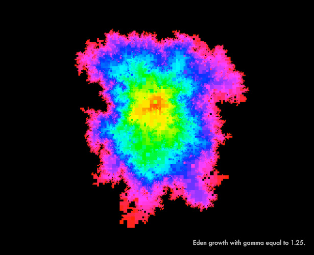
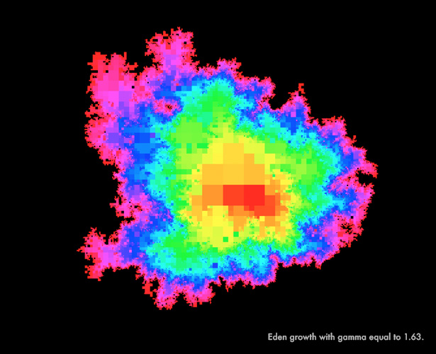
The following images show a specific random growth model, the Eden model, which describes the random growth of bacterial colonies. The colonies grow through the addition of randomly placed clusters along their boundaries. At any given point in time, it’s impossible to know for sure where on the boundary the next cluster will appear. In these images, Miller and Sheffield show how Eden growth proceeds over a random two-dimensional surface.
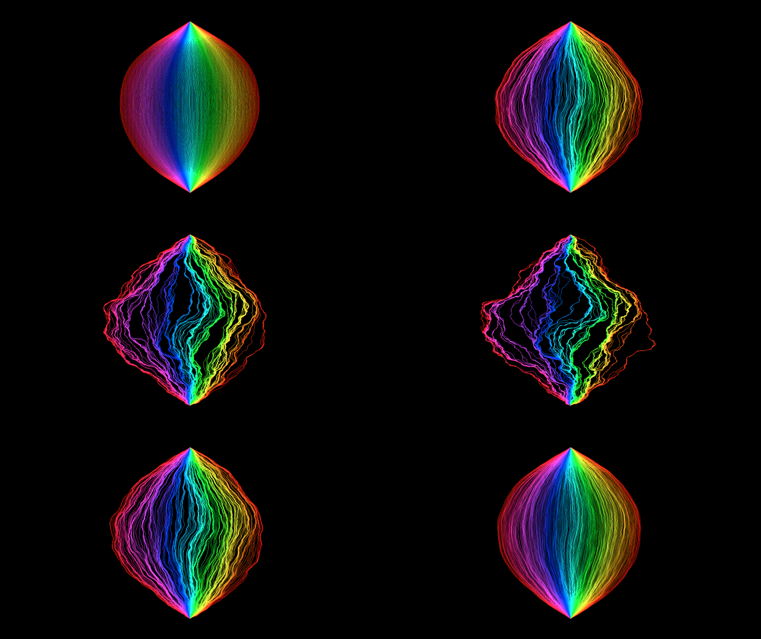
The first image shows Eden growth on a fairly flat — that is, not especially random — LQG surface. The growth proceeds in an orderly way, forming nearly concentric circles that have been color-coded to indicate the time at which growth occurs at different points on the surface.
“Figuring out how to mathematically make [random growth] rigorous is a huge stumbling block,” said Sheffield, noting that Martin Hairer of the University of Warwick won the Fields Medal in 2014 for work that overcame just these kinds of obstacles. “You always need some kind of amazing clever trick to do it.”
Random Exploration
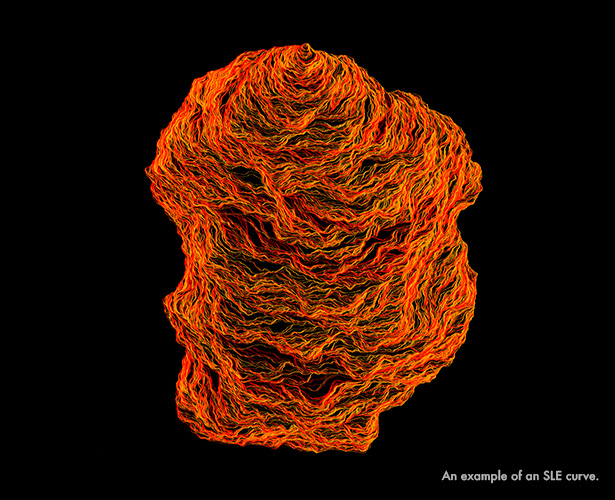
Sheffield and Miller’s clever trick is based on a special type of random one-dimensional curve that is similar to the random walk except that it never crosses itself. Physicists had encountered these kinds of curves for a long time in situations where, for instance, they were studying the boundary between clusters of particles with positive and negative spin (the boundary line between the clusters of particles is a one-dimensional path that never crosses itself and takes shape randomly). They knew these kinds of random, noncrossing paths occurred in nature, just as Robert Brown had observed that random crossing paths occurred in nature, but they didn’t know how to think about them in any kind of precise way. In 1999 Oded Schramm, who at the time was at Microsoft Research in Redmond, Washington, introduced the SLE curve (for Schramm-Loewner evolution) as the canonical noncrossing random curve.
“As a result of Schramm’s work, there were a lot of things in physics they’d known to be true in their physics way that suddenly entered the realm of things we could prove mathematically,” said Sheffield, who was a friend and collaborator of Schramm’s.
For Miller and Sheffield, SLE curves turned out to be valuable in an unexpected way. In order to measure distance on LQG surfaces, and thus show that LQG surfaces and the Brownian map were the same, they needed to find some way to model random growth on a random surface. SLE proved to be the way.
“The ‘aha’ moment was [when we realized] you can construct [random growth] using SLEs and that there is a connection between SLEs and LQG,” said Miller.
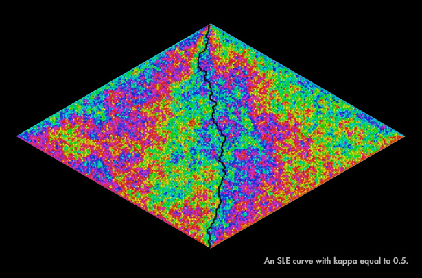
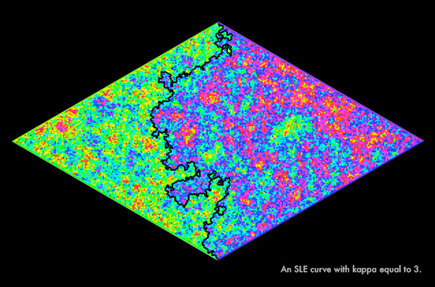
SLE curves come with a constant, kappa, which plays a similar role to the one gamma plays for LQG surfaces. Where gamma describes the roughness of an LQG surface, kappa describes the “windiness” of SLE curves. When kappa is low, the curves look like straight lines. As kappa increases, more randomness is introduced into the function that constructs the curves and the curves turn more unruly, while obeying the rule that they can bounce off of, but never cross, themselves. Here is an SLE curve with kappa equal to 0.5, followed by an SLE curve with kappa equal to 3.
Sheffield and Miller then considered a bacterial growth model, the Eden model, that had a similar effect as it advanced across a random surface: It grew in a way that “pinched off” a plot of terrain that, afterward, it never visited again. The plots of terrain cut off by the growing bacteria colony looked exactly the same as the plots of terrain cut off by the blind explorer. Moreover, the information possessed by a blind explorer at any time about the outer unexplored region of the random surface was exactly the same as the information possessed by a bacterial colony. The only difference between the two was that while the bacterial colony grew from all points on its outer boundary at once, the blind explorer’s SLE path could grow only from the tip.
In a paper posted online in 2013, Sheffield and Miller imagined what would happen if, every few minutes, the blind explorer were magically transported to a random new location on the boundary of the territory she had already visited. By moving all around the boundary, she would be effectively growing her path from all boundary points at once, much like the bacterial colony. Thus they were able to take something they could understand — how an SLE curve proceeds on a random surface — and show that with some special configuring, the curve’s evolution exactly described a process they hadn’t been able to understand, random growth. “There’s something special about the relationship between SLE and growth,” said Sheffield. “That was kind of the miracle that made everything possible.”
The distance structure imposed on LQG surfaces through the precise understanding of how random growth behaves on those surfaces exactly matched the distance structure on the Brownian map. As a result, Sheffield and Miller merged two distinct models of random two-dimensional shapes into one coherent, mathematically understood fundamental object.
Turning Randomness Into a Tool
Sheffield and Miller have already posted the first two papers in their proof of the equivalence between LQG and the Brownian map on the scientific preprint site arxiv.org; they intend to post the third and final paper later this summer. The work turned on the ability to reason across different random shapes and processes — to see how random noncrossing curves, random growth, and random two-dimensional surfaces relate to one another. It’s an example of the increasingly sophisticated results that are possible in the study of random geometry.
“It’s like you’re in a mountain with three different caves. One has iron, one has gold, one has copper — suddenly you find a way to link all three of these caves together,” said Sheffield. “Now you have all these different elements you can build things with and can combine them to produce all sorts of things you couldn’t build before.”
Many open questions remain, including determining whether the relationship between SLE curves, random growth models, and distance measurements holds up in less-rough versions of LQG surfaces than the one used in the current paper. In practical terms, the results by Sheffield and Miller can be used to describe the random growth of real phenomena like snowflakes, mineral deposits, and dendrites in caves, but only when that growth takes place in the imagined world of random surfaces. It remains to be seen whether their methods can be applied to ordinary Euclidean space, like the space we live in.
This article was reprinted on Wired.com.
